Tutorial: getting started with Delight
We will use the parameter file “tests/parametersTest.cfg”. This contains a description of the bands and data to be used. In this example we will generate mock data for the ugriz SDSS bands, fit each object with our GP using ugi bands only and see how it predicts the rz bands. This is an example for filling in/predicting missing bands in a fully bayesian way with a flexible SED model quickly via our photo-z GP.
/Users/bl/Dropbox/repos/Delight
Creating the parameter file
Let’s create a parameter file from scratch.
paramfile_txt = """
# DELIGHT parameter file
# Syntactic rules:
# - You can set parameters with : or =
# - Lines starting with # or ; will be ignored
# - Multiple values (band names, band orders, confidence levels)
#   must beb separated by spaces
# - The input files should contain numbers separated with spaces.
# - underscores mean unused column
"""
Let’s describe the bands we will use. This must be a superset (ideally the union) of all the bands involved in the training and target sets, including cross-validation.
Each band should have its own file, containing a tabulated version of the filter response.
See example files shipped with the code for formatting.
paramfile_txt += """
[Bands]
names: U_SDSS G_SDSS R_SDSS I_SDSS Z_SDSS
directory: data/FILTERS
"""
Let’s now describe the system of SED templates to use (needed for the mean fct of the GP, for simulating objects, and for the template fitting routines).
Each template should have its own file (see shipped files for formatting example).
lambdaRef will be the pivot wavelenght used for normalizing the templates.
p_z_t and p_t containts parameters for the priors of each template, for p(z|t) p(t).
Calibrating those numbers will be the topic of another tutorial.
By default the set of templates and the prior calibration can be left untouched.
paramfile_txt += """
[Templates]
directory: ./data/CWW_SEDs
names: El_B2004a Sbc_B2004a Scd_B2004a SB3_B2004a SB2_B2004a Im_B2004a ssp_25Myr_z008 ssp_5Myr_z008
p_t: 0.27 0.26 0.25 0.069 0.021 0.11 0.0061 0.0079
p_z_t:0.23 0.39 0.33 0.31 1.1 0.34 1.2 0.14
lambdaRef: 4.5e3
"""
The next section if for simulating a photometric catalogue from the templates.
catalog files (trainingFile, targetFile) will be created, and have the adequate format for the later stages.
noiseLevel describes the relative error for the absolute flux in each band.
paramfile_txt += """
[Simulation]
numObjects: 1000
noiseLevel: 0.03
trainingFile: data/galaxies-fluxredshifts.txt
targetFile: data/galaxies-fluxredshifts2.txt
"""
We now describe the training file.
catFile is the input catalog. This should be a tab or space
separated file with numBands + 1 columns.
bandOrder describes the ordering of the bands in the file.
Underscore _ means an ignored column, for example a band that
shouldn’t be used. The band names must correspond to those in the filter
section.
redshift is for the photometric redshift. referenceBand is the
reference band for normalizing the fluxes and luminosities.
extraFracFluxError is an extra relative error to add in quadrature
to the flux errors.
paramFile will contain the output of the GP applied to the training
galaxies, i.e. the minimal parameters that must be stored in order to
reconstruct the fit of each GP.
crossValidate is a flag for performing optional cross-validation. If
so, CVfile will contain cross-validation data.
crossValidationBandOrder is similar to bandOrder and describes
the bands to be used for cross-validation. In this example I have left
the R band out of bandOrder and put it in
crossValidationBandOrder. However, this feature won’t work on
simulated data, only on real data (i.e., the simulateWithSEDs script
below does not generate cross-validation bands).
numChunks is the number of chunks to split the training data into.
At present please stick to 1.
paramfile_txt += """
[Training]
catFile: data/galaxies-fluxredshifts.txt
bandOrder: U_SDSS U_SDSS_var G_SDSS G_SDSS_var _ _ I_SDSS I_SDSS_var Z_SDSS Z_SDSS_var redshift
referenceBand: I_SDSS
extraFracFluxError: 1e-4
paramFile: data/galaxies-gpparams.txt
crossValidate: False
CVfile: data/galaxies-gpCV.txt
crossValidationBandOrder: _ _ _ _ R_SDSS R_SDSS_var _ _ _ _ _
numChunks: 1
"""
The section of the target catalog has very similar structure and
parameters. The catFile, bandOrder, referenceBand, and
extraFracFluxError have the same meaning as for the training, but of
course don’t have to be the same.
redshiftpdfFile and redshiftpdfFileTemp will contain tabulated
redshift posterior PDFs for the delight-apply and templateFitting
scripts.
Similarly, metricsFile and metricsFileTemp will contain metrics
calculated from the PDFs, like mean, mode, etc. This is particularly
informative if redshift is also provided in the target set.
The compression mode can be activated with useCompression and will
produce new redshift PDFs in the file redshiftpdfFileComp, while
compressIndicesFile and compressMargLikFile will contain the
indices and marginalized likelihood for the objects that were kept
during compression. The number of objects is controled with
Ncompress.
paramfile_txt += """
[Target]
catFile: data/galaxies-fluxredshifts2.txt
bandOrder: U_SDSS U_SDSS_var G_SDSS G_SDSS_var _ _ I_SDSS I_SDSS_var Z_SDSS Z_SDSS_var redshift
referenceBand: I_SDSS
extraFracFluxError: 1e-4
redshiftpdfFile: data/galaxies-redshiftpdfs.txt
redshiftpdfFileTemp: data/galaxies-redshiftpdfs-cww.txt
metricsFile:  data/galaxies-redshiftmetrics.txt
metricsFileTemp:  data/galaxies-redshiftmetrics-cww.txt
useCompression: False
Ncompress: 10
compressIndicesFile: data/galaxies-compressionIndices.txt
compressMargLikFile: data/galaxies-compressionMargLikes.txt
redshiftpdfFileComp: data/galaxies-redshiftpdfs-comp.txt
"""
Finally, there are various other parameters related to the method itself.
The (hyper)parameters of the Gaussian process are zPriorSigma,
ellPriorSigma (locality of the model predictions in redshift and
luminosity), fluxLuminosityNorm (some normalization parameter),
alpha_C, alpha_L, V_C, V_L (smoothness and variance of
the latent SED model), lines_pos, lines_width (positions and
widths of the lines in the latent SED model).
redshiftMin, redshiftMax, and redshiftBinSize describe the
linear fine redshift grid to compute PDFs on.
redshiftNumBinsGPpred describes the granuality (in log scale!) for
the GP kernel to be exactly calculated on; it will then be interpolated
on the finer grid.
redshiftDisBinSize is the binsize for a tomographic redshift
binning.
confidenceLevels are the confidence levels to compute in the
redshift PDF metrics.
The values below should be a good default set for all of those parameters.
paramfile_txt += """
[Other]
rootDir: ./
zPriorSigma: 0.2
ellPriorSigma: 0.5
fluxLuminosityNorm: 1.0
alpha_C: 1.0e3
V_C: 0.1
alpha_L: 1.0e2
V_L: 0.1
lines_pos: 6500 5002.26 3732.22
lines_width: 20.0 20.0 20.0
redshiftMin: 0.1
redshiftMax: 1.101
redshiftNumBinsGPpred: 100
redshiftBinSize: 0.001
redshiftDisBinSize: 0.2
confidenceLevels: 0.1 0.50 0.68 0.95
"""
Let’s write this to a file.
with open('tests/parametersTest.cfg','w') as out:
    out.write(paramfile_txt)
Running Delight
Processing the filters and templates, and create a mock catalog
First, we must fit the band filters with a gaussian mixture. This is done with this script:
U_SDSS
G_SDSS
R_SDSS
I_SDSS
Z_SDSS
Second, we will process the library of SEDs and project them onto the filters, (for the mean fct of the GP) with the following script (which may take a few minutes depending on the settings you set):
Third, we will make some mock data with those filters and SEDs:
Train and apply
Run the scripts below. There should be a little bit of feedback as it is going through the lines. For up to 1e4 objects it should only take a few minutes max, depending on the settings above.
--- TEMPLATE FITTING ---
Thread number / number of threads:  1 1
Input parameter file: tests/parametersTest.cfg
Number of Target Objects 1000
Thread  0  analyzes lines  0  to  1000
--- DELIGHT-LEARN ---
Number of Training Objects 1000
Thread  0  analyzes lines  0  to  1000
--- DELIGHT-APPLY ---
Number of Training Objects 1000
Number of Target Objects 1000
Thread  0  analyzes lines  0  to  1000
0 0.1311957836151123 0.014869213104248047 0.013804912567138672
100 0.06870007514953613 0.006330966949462891 0.004736900329589844
200 0.10263180732727051 0.008839130401611328 0.011183977127075195
300 0.07733988761901855 0.007596015930175781 0.007447004318237305
400 0.07348513603210449 0.006279945373535156 0.006253957748413086
500 0.07892394065856934 0.007573127746582031 0.014636993408203125
600 0.0829770565032959 0.0071430206298828125 0.0066449642181396484
700 0.11001420021057129 0.008404970169067383 0.007412910461425781
800 0.1179349422454834 0.009317159652709961 0.011492013931274414
900 0.13953113555908203 0.012920856475830078 0.010159015655517578
Analyze the outputs
# First read a bunch of useful stuff from the parameter file.
params = parseParamFile('tests/parametersTest.cfg', verbose=False)
bandCoefAmplitudes, bandCoefPositions, bandCoefWidths, norms\
    = readBandCoefficients(params)
bandNames = params['bandNames']
numBands, numCoefs = bandCoefAmplitudes.shape
fluxredshifts = np.loadtxt(params['target_catFile'])
fluxredshifts_train = np.loadtxt(params['training_catFile'])
bandIndices, bandNames, bandColumns, bandVarColumns, redshiftColumn,\
            refBandColumn = readColumnPositions(params, prefix='target_')
redshiftDistGrid, redshiftGrid, redshiftGridGP = createGrids(params)
dir_seds = params['templates_directory']
dir_filters = params['bands_directory']
lambdaRef = params['lambdaRef']
sed_names = params['templates_names']
nt = len(sed_names)
f_mod = np.zeros((redshiftGrid.size, nt, len(params['bandNames'])))
for t, sed_name in enumerate(sed_names):
    f_mod[:, t, :] = np.loadtxt(dir_seds + '/' + sed_name + '_fluxredshiftmod.txt')
# Load the PDF files
metricscww = np.loadtxt(params['metricsFile'])
metrics = np.loadtxt(params['metricsFileTemp'])
# Those of the indices of the true, mean, stdev, map, and map_std redshifts.
i_zt, i_zm, i_std_zm, i_zmap, i_std_zmap = 0, 1, 2, 3, 4
i_ze = i_zm
i_std_ze = i_std_zm

pdfs = np.loadtxt(params['redshiftpdfFile'])
pdfs_cww = np.loadtxt(params['redshiftpdfFileTemp'])
pdfatZ_cww = metricscww[:, 5] / pdfs_cww.max(axis=1)
pdfatZ = metrics[:, 5] / pdfs.max(axis=1)
nobj = pdfatZ.size
#pdfs /= pdfs.max(axis=1)[:, None]
#pdfs_cww /= pdfs_cww.max(axis=1)[:, None]
pdfs /= np.trapz(pdfs, x=redshiftGrid, axis=1)[:, None]
pdfs_cww /= np.trapz(pdfs_cww, x=redshiftGrid, axis=1)[:, None]
ncol = 4
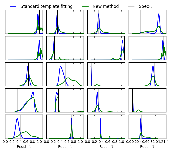
fig, axs = plt.subplots(5, ncol, figsize=(7, 6), sharex=True, sharey=False)
axs = axs.ravel()
z = fluxredshifts[:, redshiftColumn]
sel = np.random.choice(nobj, axs.size, replace=False)
lw = 2
for ik in range(axs.size):
k = sel[ik]
print(k, end=" ")
axs[ik].plot(redshiftGrid, pdfs_cww[k, :],lw=lw, label='Standard template fitting')# c="#2ecc71",
axs[ik].plot(redshiftGrid, pdfs[k, :], lw=lw, label='New method') #, c="#3498db"
axs[ik].axvline(fluxredshifts[k, redshiftColumn], c="k", lw=1, label=r'Spec-$z$')
ymax = np.max(np.concatenate((pdfs[k, :], pdfs_cww[k, :])))
axs[ik].set_ylim([0, ymax*1.2])
axs[ik].set_xlim([0, 1.1])
axs[ik].set_yticks([])
axs[ik].set_xticks([0.0, 0.2, 0.4, 0.6, 0.8, 1.0, 1.2, 1.4])
for i in range(ncol):
axs[-i-1].set_xlabel('Redshift', fontsize=10)
axs[0].legend(ncol=3, frameon=False, loc='upper left', bbox_to_anchor=(0.0, 1.4))
fig.tight_layout()
fig.subplots_adjust(wspace=0.1, hspace=0.1, top=0.96)
569 381 281 54 883 76 253 910 73 297 813 155 744 473 89 582 571 762 414 627
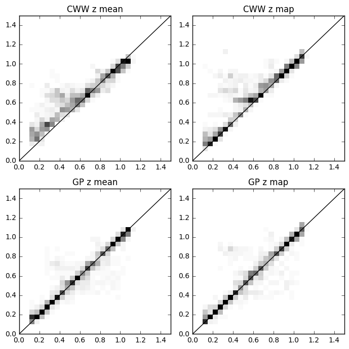
fig, axs = plt.subplots(2, 2, figsize=(7, 7))
zmax = 1.5
rr = [[0, zmax], [0, zmax]]
nbins = 30
h = axs[0, 0].hist2d(metricscww[:, i_zt], metricscww[:, i_zm], nbins, cmap='Greys', range=rr)
hmin, hmax = np.min(h[0]), np.max(h[0])
axs[0, 0].set_title('CWW z mean')
axs[0, 1].hist2d(metricscww[:, i_zt], metricscww[:, i_zmap], nbins, cmap='Greys', range=rr, vmax=hmax)
axs[0, 1].set_title('CWW z map')
axs[1, 0].hist2d(metrics[:, i_zt], metrics[:, i_zm], nbins, cmap='Greys', range=rr, vmax=hmax)
axs[1, 0].set_title('GP z mean')
axs[1, 1].hist2d(metrics[:, i_zt], metrics[:, i_zmap], nbins, cmap='Greys', range=rr, vmax=hmax)
axs[1, 1].set_title('GP z map')
axs[0, 0].plot([0, zmax], [0, zmax], c='k')
axs[0, 1].plot([0, zmax], [0, zmax], c='k')
axs[1, 0].plot([0, zmax], [0, zmax], c='k')
axs[1, 1].plot([0, zmax], [0, zmax], c='k')
fig.tight_layout()
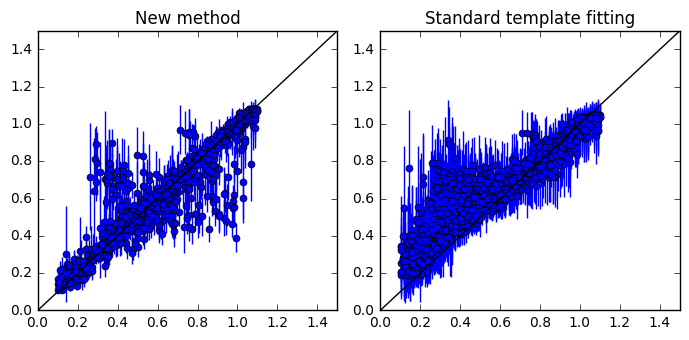
fig, axs = plt.subplots(1, 2, figsize=(7, 3.5))
chi2s = ((metrics[:, i_zt] - metrics[:, i_ze])/metrics[:, i_std_ze])**2

axs[0].errorbar(metrics[:, i_zt], metrics[:, i_ze], yerr=metrics[:, i_std_ze], fmt='o', markersize=5, capsize=0)
axs[1].errorbar(metricscww[:, i_zt], metricscww[:, i_ze], yerr=metricscww[:, i_std_ze], fmt='o', markersize=5, capsize=0)
axs[0].plot([0, zmax], [0, zmax], 'k')
axs[1].plot([0, zmax], [0, zmax], 'k')
axs[0].set_xlim([0, zmax])
axs[1].set_xlim([0, zmax])
axs[0].set_ylim([0, zmax])
axs[1].set_ylim([0, zmax])
axs[0].set_title('New method')
axs[1].set_title('Standard template fitting')

fig.tight_layout()
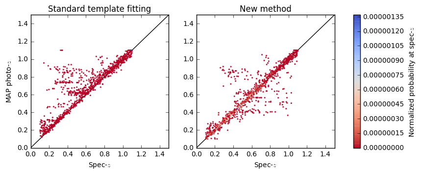
cmap = "coolwarm_r"
vmin = 0.0
alpha = 0.9
s = 5
fig, axs = plt.subplots(1, 2, figsize=(10, 3.5))
vs = axs[0].scatter(metricscww[:, i_zt], metricscww[:, i_zmap],
                    s=s, c=pdfatZ_cww, cmap=cmap, linewidth=0, vmin=vmin, alpha=alpha)
vs = axs[1].scatter(metrics[:, i_zt], metrics[:, i_zmap],
                    s=s, c=pdfatZ, cmap=cmap, linewidth=0, vmin=vmin, alpha=alpha)
clb = plt.colorbar(vs, ax=axs.ravel().tolist())
clb.set_label('Normalized probability at spec-$z$')
for i in range(2):
    axs[i].plot([0, zmax], [0, zmax], c='k', lw=1, zorder=0, alpha=1)
    axs[i].set_ylim([0, zmax])
    axs[i].set_xlim([0, zmax])
    axs[i].set_xlabel('Spec-$z$')
axs[0].set_ylabel('MAP photo-$z$')

axs[0].set_title('Standard template fitting')
axs[1].set_title('New method')
<matplotlib.text.Text at 0x11dc77a20>
Conclusion
Don’t be too harsh with the results of the standard template fitting or the new methods since both have a lot of parameters which can be optimized!
If the results above made sense, i.e. the redshifts are reasonnable for both methods on the mock data, then you can start modifying the parameter files and creating catalog files containing actual data! I recommend using less than 20k galaxies for training, and 1000 or 10k galaxies for the delight-apply script at the moment. Future updates will address this issue.